Predicting Stock Prices using Machine learning

The world of finance contains LOTS of data. This makes finance a very suitable subject to be used in Machine Learning. In this case I’ve decided to investigate further if it is possible to predict the stock market data as the data is readily available. In this case I’ve selected a couple of stocks / Exchange Traded Funds (ETF) to find out if the selected Machine Learning Models are suitable for the broader based index (which tends to be more stable) or for stocks (higher volatility).

Link to notebook: Jupyter Notebook (stock_prediction)

ETF / Stocks Selected

• SPY
• MSFT
• GOOGL
• AMZN

Obtaining the Data

The data will be obtained from AlphaVantage for the Stock Data from Daily Adjusted. The Daily Adjusted price accounts for the difference for any stock splits and dividends paid out during the selected time frame selected.

We will be storing all the tickers in a DataFrame df_stocks to make it easy to perform the calculations on each DataFrame during Feature Engineering.

list_stocks = ['SPY', 'MSFT', 'GOOGL', 'AMZN']

def get_stock_price(ticker):
  """
  Returns the Stock Data as a DataFrame.
  Note: The API Key is declared separately and used in this function.
  """
  url_address = 'https://www.alphavantage.co/query'
  func_name = 'TIME_SERIES_DAILY_ADJUSTED'
  output_size = 'full'

    res = requests.get(url_address,
                params = dict(function = func_name,
                             symbol = ticker,
                             outputsize = output_size,
                             apikey = API_KEY))
    res_json = res.json()
    return pd.DataFrame(res_json['Time Series (Daily)']).transpose()

df_stocks = [get_stock_price(stock) for stock in list_stocks]

Exploratory Data Analysis

In this example we will use SPY(S&P 500) as an example to perform EDA in this blog post *Assumptions: MSFT, GOOGL and AMZN will have similar performance based on SPY**.

Some questions we can answer from EDA:

• Is there any trend to the data (up, down or range-bound)
• Is there any seasonality in price movement within each week (Monday to Friday)
• Is there any seasonality in price movement within each month (01 to 31)
• Is there any seasonality in price movement within the year (Jan to December)

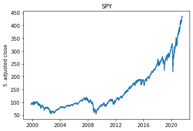
Using SPY as an Example, we will perform box and line plots to find out if there is any trends that can be observed from the data (does Jan have a larger postive stock movement etc.)

Check for Trend

Check for Seasonality

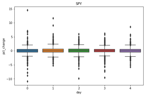
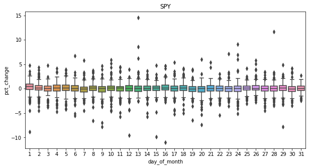
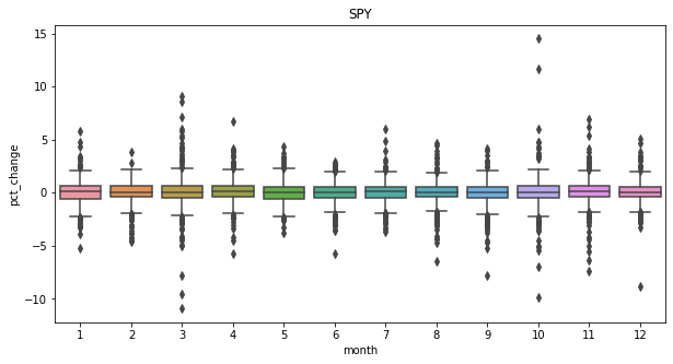
From the 3 plots above we can see that on average there is no seasonality between the day of the week, time of the month and time of the year when the stocks are being traded and that overtime stocks go up! Which is a good thing for investors.

Feature Engineering

When a stock is being traded, technical indicators are used by traders to signal when to buy or sell a stock. These technical indicators are calculated from the historical stock price. In our model we will be including the indicator of Simple Moving Average (50 days & 200 days).

Simple Moving Average

To calculate the Simple Moving Average, we will be using the function .rolling() to compute the simple moving average. The documentation of the function can be found here.

for stock in df_stocks:
    stock['SMA50'] = stock['5. adjusted close'].rolling(window = 50).mean()
    stock['SMA200'] = stock['5. adjusted close'].rolling(window = 200).mean()

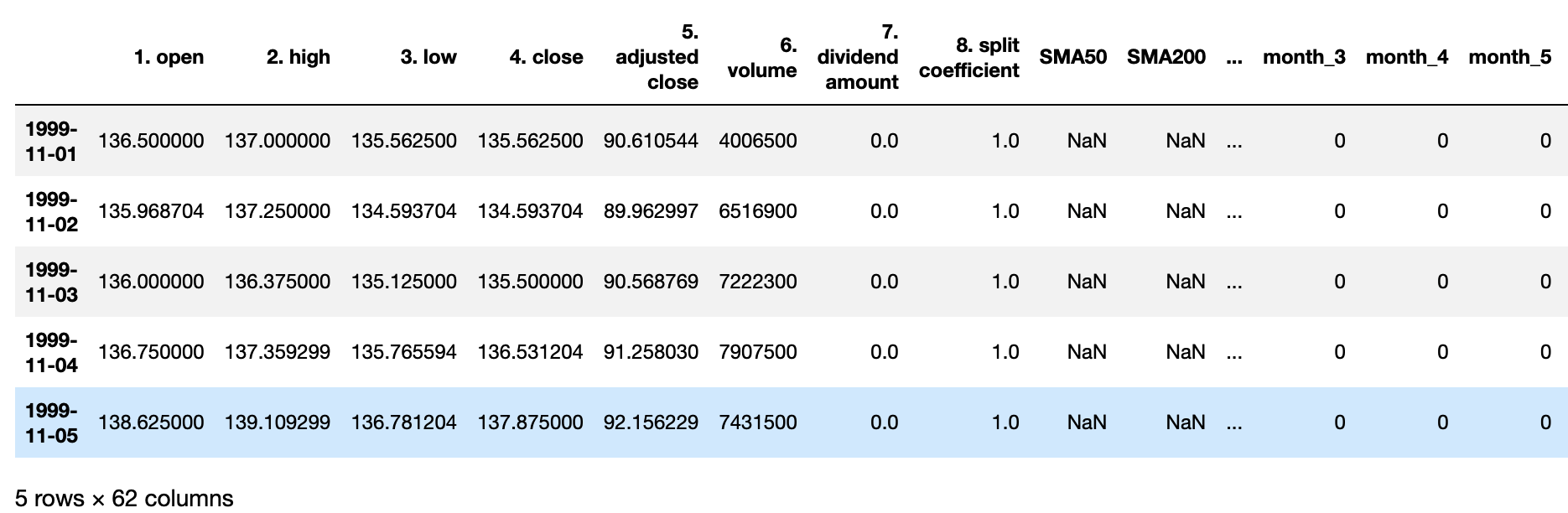
Data Dummification

We will be extracting additional infomration from our data that will be used in training the model. These are the day, day_of_month, and month information from the index with the results as follows with 61 columns. Note: First 5 rows for SMA50 and SMA200 shows NaN from the computation of the moving averages

Selecting the Time Period

For our case we will be selecting the time period of 01-Jan-2017 to 31-June-2021. This should give sufficient data points to train the model and forecast the prices.

Splitting the Data

For most models that split their data into train and test, we will use sklearn.model_selection.train_test_split(). By using train_test_split it means that we are randomly sampling the data which is not appropriate for time-series modelling where the past results will have an impact on future forecasts. Therefore in our case where Time-series is used, we will be splitting it using the length of the DataFrame.

train_test_split

How train_test_split() selects the data

Time-series split

We will be splitting the data as shown in the above illustration. Since we are storing the stock data in a list, we will loop through them to get the train and test data which will then be fitted to the selected models.

for stock_name, stock in enumerate(ml_stocks):
    y = stock['5. adjusted close']
    X = stock.drop(['5. adjusted close'], axis = 1)
    # Split into train and test
    X_train = X.iloc[:int(0.8*len(X))]
    y_train = y.iloc[:int(0.8*len(y))]

    X_test = X.iloc[int(0.8*len(X)):]
    y_test = y.iloc[int(0.8*len(y)):]

Machine Learning Models

We will be using several Machine Learning models to evaluate their performance for the time-series prediction

• Linear Regression
• Decision Tree Regressor
• Random Forest Regressor

The following models are trained with each of the stocks. As each stock behaves differently, each model will be trained and used to predict for that specific stock.

Model Evaluation

As this is a regression model, for Model evaluation we will be performed using the following metrics:

• R²
• Root Mean Squared Error(RMSE)

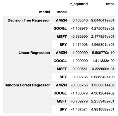
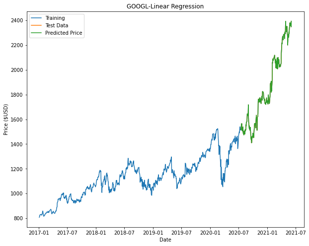
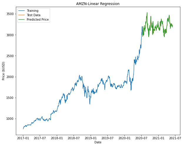
From the results shown, it can be seen that Linear Regression gives us the best R² value and RMSE values compared to the other predictors.

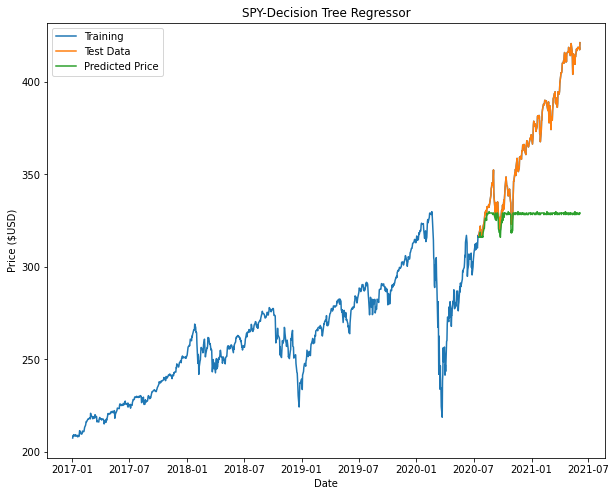
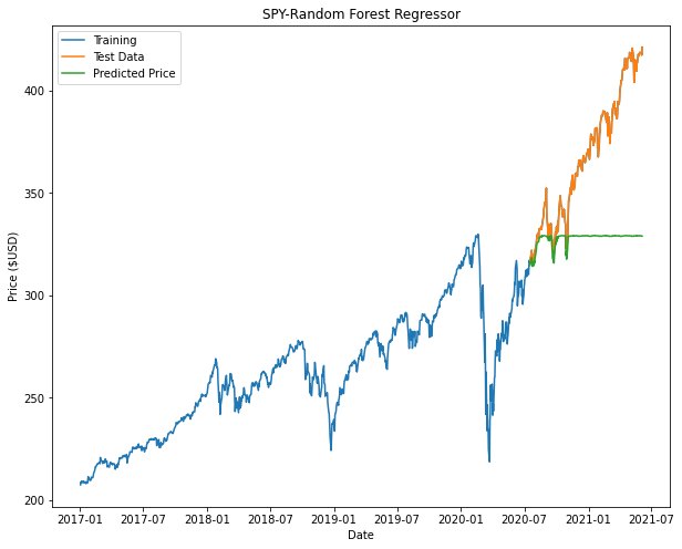
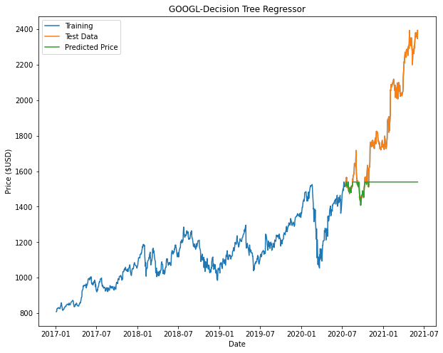
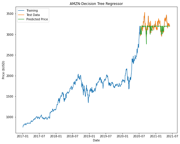
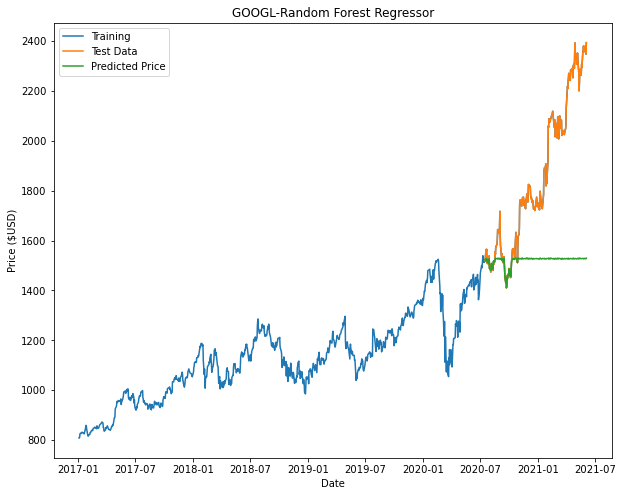
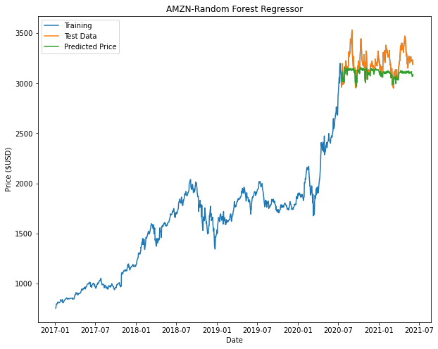
From the plots we can see that both Decision Tree and Random Forest appears to taper off halfway or at the beginning of the prediction. This is attributed to factors such as insufficient nodes in the model to give us an accurate prediction.

Results of SPY below: Linear Regression (SPY)

Decision Tree Regressor (SPY)

Random Forest Regressor (SPY)

Summary of plots (MSFT, GOOGL, AMZN) using 3 different Machine Learning Models

	Microsoft (MSFT)	Google (GOOGL)	Amazon (AMZN)
Linear Regression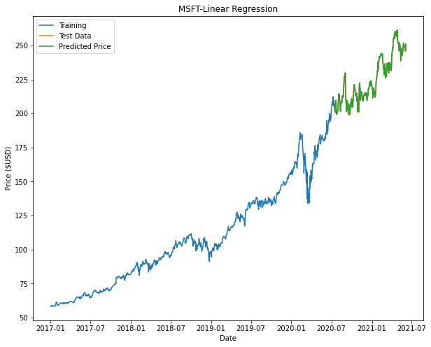
Decision Tree Regressor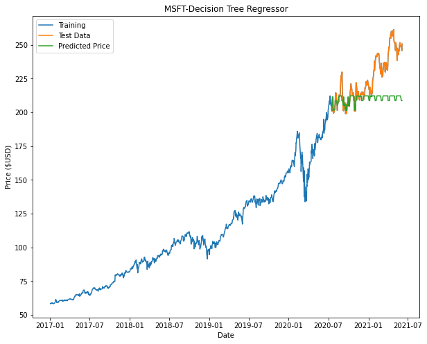
Random Forest Regressor

Conclusion

Based on the results, Linear Regression returns the best model. It is noted that in our models for Decision Tree and Random Forest there may not be enough nodes to accurately predict the price (This can be seen with some of the flat-lining of the predicted data.). In order to improve these models, we can include additional parameters and tune the hyperparameters of these models to have a better fit.

Further Improvements

In order to further improve the model, Principal Component Analysis (PCA) can be used to reduce the dimensions of the inputs and to include additional technical indicators such as RSI or MACD that are commonly used in trading.